Entry
The HLDS pipeline turns a multichannel time-series recording into a stack of hidden trajectories: x, a filtered copy of the observation y, then u (16 dimensions), then z (2 dimensions) at the top. The data are a collaborator's dataset of 27 recordings, each trial carrying one of three condition labels. The tempting test is a classifier on z that beats chance.
It is the wrong test. Every layer is a function of y, so anything a probe reads from z was already in y. The question that matters is narrower: does a layer carry condition information beyond its own input, in a form that is easier to read, and does that hold on recordings the analysis never touched? This post covers the protocol I built to answer it and the first three rounds. No round produced a layer that beat its input.
The protocol, written before the runs
- Block folds. Each recording is cut into five contiguous segments, so test trials are never interleaved with training trials. That makes it much harder for slow drift to pass as decoding.
- A design null. Chance is not taken to be 1/3. Each null draw relabels a recording's trials with another recording's real condition sequence (or, in 13 of the 280 draws across the 14 explore recordings, a block rotation of one), while the fold partition stays fixed. A row's own delta is its balanced accuracy minus that recording's null mean.
- An explore/confirm split. 14 recordings for exploring and 13 held back, split with a fixed seed and stratified on a baseline's per-recording score. The goal I froze before round 2 added that each configuration gets at most one confirm run, declared in the ledger first.
- The screen. The rows are layer × summary (covariance or band-power of the trajectory; "cov" and "bandpower" in the figure) × probe (shrinkage linear discriminant analysis, written shrinkage LDA, or logistic regression; "slda" and "lr"). The paired delta d is layer minus y on the same summary and probe, per recording. A layer passes if, on its best row by d, d ≥ 0 and its own delta is positive at two-sided p < 0.05.
- An input gate. Before any HLDS is trained on a new input, that input is probed alone. It passes if, on whichever of its four rows does best against the reference input, the mean paired difference is above zero.
The reference input is 20 channels summed into one signal, split into four frequency bands with 16 lags each: 64 columns. On the explore set it is a weak carrier. Its strongest row, covariance with shrinkage LDA, reaches own +0.040 (p 0.09), and only band-power with logistic regression clears p < 0.05 (+0.027, p 0.042).
Round 0: six inputs and the default model
I probed six candidate inputs first. All six passed the gate, including one that sat below the reference on three of its four rows. Keeping channels separate gave the largest paired gain, +0.052 (p 0.044), and four spatial principal components gave the largest own delta, +0.075 (p 0.0014). No paired gain survives correction over the 24 input rows. A gate that everything passes is not filtering anything. Only one input was judged both worth training and affordable in round 1, the multi-modal one below: separate channels exceed the trainer's input size, four spatial components would have cost an estimated 37 times the default model, and two components were deferred on a weak gain and an estimated, never measured, cost of about 5.6 times.
The default HLDS on the reference input failed the screen. u's best row had d −0.023 and own +0.008 (p 0.69); z's had d −0.026 and own +0.005 (p 0.75). Some rows were nominally significantly worse than y: z band-power with logistic regression had d −0.047 (p 0.008). The diagnostics suggested why: u and z had about one effective dimension within a trial (participation ratio 1.06-1.10, against 5.15 for y), and trials looked more alike in the layers than in the input.
Round 1: five noise settings and a multi-modal arm
The obvious knob was the noise hierarchy. By default each layer's process noise is ten times smaller than the one below (σz 0.001, σu 0.01, σx 0.1, with observation noise σy 1), so I gave the upper layers more noise to let them move. I ran five settings plus a multi-modal arm that adds a second recorded signal to the input (11 recordings had enough usable coverage of it).
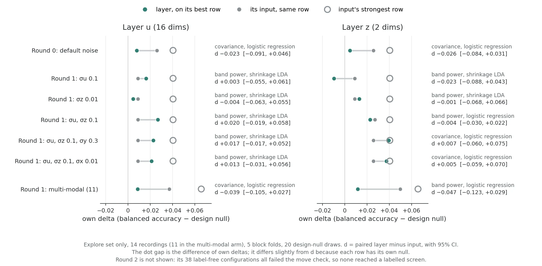
Raising the noise brought most best rows closer to the input: across the five settings, best-row d ranged from −0.023 to +0.020. The largest, +0.020, was for u with both upper noises at 0.1, with a 95% CI of −0.019 to +0.058. No best row reached own p < 0.05; the closest was z in the inverted setting (σx lowered to 0.01, σu and σz raised to 0.1), at 0.052. With best-row selection over seven configurations and two layers, about 0.7 to 1 false pass would be expected by chance alone; none occurred. The open circles show a second point: selecting the best row by d favours rows where the input is weak. The input's own strongest row (+0.040, or +0.066 with p 0.033 for the multi-modal input) sat at or above every layer's best row. Off the best rows, two z covariance rows with shrinkage LDA did clear own p < 0.05 (+0.043, p 0.034, and +0.034, p 0.042), but both had a negative paired d against the input on the same row (−0.006 and −0.012): above chance is not beyond the input. In the multi-modal arm both layers fell below the input (d −0.039 and −0.047).
In the default and multi-modal models the point estimates sat below the input, though not significantly on the best rows; under raised noise the best rows sat near the input, never significantly above it. Across all seven, no layer significantly beat its input. At n = 14 this is absence of evidence, and best-row gains of about +0.06 to +0.07 cannot be excluded.
The rows that looked like a lead
Outside the pre-registered family, log-variance rows of the layers looked good: u in the inverted setting reached own +0.055 (p 0.003) with logistic regression. They could not count, but I checked them afterwards, on the explore set only, against unsupervised controls of the same size: the log-variance of 16 principal components of the input for u, 2 for z, fitted on training trials, and random projections of the same sizes. With the same probe, the 16-component control alone reached own +0.053 (p 0.014), and +0.074 (p 0.008) with shrinkage LDA. Layer minus its matched control ranged from −0.035 to +0.033, with every p ≥ 0.16. Against the input's own covariance row the layer rows were within ±0.02 (every p ≥ 0.53): they cleared p < 0.05 where that row did not, a difference in significance, not in accuracy. This is what projecting to a few dimensions gives without any dynamics, though paired intervals about ±0.05 wide leave differences of that size open. The matched principal-component control became a required comparison in the redesign.
Round 2: nothing moved, so nothing was screened
Before round 2 I froze a goal and a stop rule, and made a label-free move check binding: on two explore recordings and one fold, u or z needs within-trial participation ratio ≥ 1.5 and between-trial band-power spread ≥ 0.35 before it may see labels. 38 configurations covered every knob on the menu: the reset prior, no reset, smoothed states and a learned observation matrix. None moved. The stop rule fired on its first condition, and the confirm set was never used.
The label-free diagnosis that followed, in the next post, found the first part of the reason: the summed input has roughly one slow direction, so the layers had little to spread into.